Onward to Movement!
In part one, we looked at some fundamentals about handling images in python, specifically with NumPy arrays and the scikit-image library. We now continue forward, and explore some of the processes we’ll use to augment our image based dataset. We’ll look at each process in isolation to understand how it works before we implement them together to generate / augment modified images.
In part one, we looked at some fundamentals about handling images in python, specifically with NumPy arrays and the scikit-image library. We now continue forward, and explore some of the processes we’ll use to augment our image based dataset. We’ll look at each process in isolation to understand how it works before we implement them together to generate / augment modified images.
import numpy as np #numpy represents complex dimensional data as arrays

import matplotlib.pyplot as plt #some standard python plotting

import skimage #our imaging library
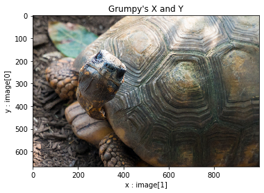
grump = skimage.io.imread('turtle.jpg') #load up our grumpy tortoise-guide
adapthist = skimage.exposure.equalize_adapthist(skimage.color.rgb2gray(grump), clip_limit = .2) #and let's enhance
Translation
X-Y movement when working in scikit-image is not quite as straightforward as you’d think on first glance. Remember, the pixel location [0, 0] corresponds to the top left of the image, not, as you might think and I constantly have to remind myself, the bottom left.
Transformations in scikit can be done in a few different ways, but one of the most useful, if difficult to tame, is the warp matrix. A warp matrix, in scikit, is an INVERSE homogeneous transformation matrix structured in a 3×3 format, to accommodate extra data dimensions for color channels. That means in order to translate an image by, say, 250 pixels to the right and 250 pixels down, you must supply your transformation values as the inverse: -250 x and -250 y.
These matrices be built by functions and contained in a specific object type, such as the return from
SimilarityTransform, or they can be built by hand as a numpy matrix.
The resulting matrix for a translation will be structured like this:
\begin{bmatrix} 1 & 0 & X value \\ 0 & 1 & Y value \\ 0 & 0 & 1 \end{bmatrix}#let's move the image to the right and down :
translatex, translatey = -250, -100
#creating an inverse matrix to move the image by our translate values
matrix = np.matrix([[1, 0, translatex],
[0,1,translatey],
[0,0,1]]
)
print('our inverse matrix : \n', matrix)
#to apply a transformation matrix, we use the skimage.transform.warp function
moved_grump = skimage.transform.warp(adapthist, matrix)
#and scoot Grump back to the original position by making an inverted-inverse matrix. It does make sense, I promise.
matrix = np.matrix([[1, 0, -1*translatex],
[0,1,-1*translatey],
[0,0,1]]
)
restored_grump = skimage.transform.warp(moved_grump, matrix)
plt.figure(figsize = (18, 8))
plt.subplot(1,3,1)
plt.imshow(moved_grump, cmap = 'gray')
plt.title('Grump translated by x and y')
plt.subplot(1,3,2)
plt.imshow(restored_grump, cmap = 'gray')
plt.title('Grump translated back to org coordiantes')
plt.subplot(1,3,3)
plt.imshow(adapthist + restored_grump, cmap = 'gray')
plt.title('Grump org PLUS restored, just to prove a point')
plt.show()

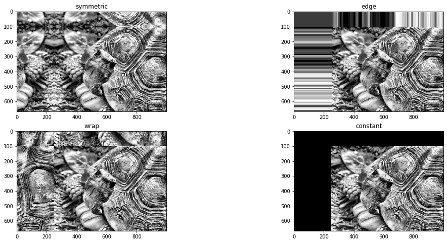
When translating, we have several options of how to deal with the blank areas created by moving the
image. These are handled by the mode argument to the warp function. Let’s use the same
transform matrix and warp function, and see what the different modes of warping change the image.
Some of these will be more useful than others, some will let you preserve data outside the new
boundaries that would be lost – again, they all have a place and use case, but constant
will most likely be your go-to for a lot of those science-style situations.
translatex, translatey = -250, -100
matrix = np.matrix([[1, 0, translatex],
                    [0,1,translatey],
                    [0,0,1]]
                  )

symmetric_grump = skimage.transform.warp(adapthist, matrix, mode ='symmetric')

edge_grump = skimage.transform.warp(adapthist, matrix, mode ='edge')

wrap_grump = skimage.transform.warp(adapthist, matrix, mode ='wrap')

constant_grump = skimage.transform.warp(adapthist, matrix, mode ='constant')

plt.figure(figsize = (18, 8))
plt.subplot(2,2,1)
plt.imshow(symmetric_grump, cmap = 'gray')
plt.title('symmetric')
plt.subplot(2,2,2)
plt.imshow(edge_grump, cmap = 'gray')
plt.title('edge')
plt.subplot(2,2,3)
plt.imshow(wrap_grump, cmap = 'gray')
plt.title('wrap')
plt.subplot(2,2,4)
plt.imshow(constant_grump, cmap = 'gray')
plt.title('constant')
plt.show()
Rotation
Now, we could use the same transformation type to create image roation, using an inverse matrix to rotate the image by Θ theta degrees:
\begin{bmatrix} cos\theta & sin\theta & 0 \\ -sin\theta & cos\theta & 0 \\ 0 & 0 & 1 \end{bmatrix}
But we have a whole toolkit, so let’s look at something different!
We have a built-in function in the transform module, called… you’ll never guess it. ROTATE!
Sorry, I know I ruined the suspense.transform.rotate will take the image and an angle
argument, and return the rotated image!
note – the rotate function’s angle argument will transform in degrees with positive
values moving counter-clockwise
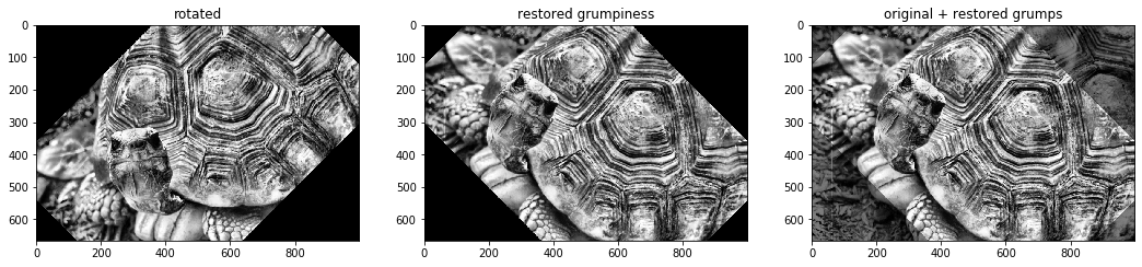
#spin your grump-tortoise round and round!
rotate_grump = skimage.transform.rotate(adapthist, angle = 45, mode = 'constant', resize = False)
restored_grump = skimage.transform.rotate(rotate_grump, angle = -45, mode = 'constant', resize = False)
composite_grump = adapthist + restored_grump

plt.figure(figsize = (18, 8))
plt.subplot(1,3,1)
plt.imshow(rotate_grump, cmap = 'gray')
plt.title('rotated')
plt.subplot(1,3,2)
plt.imshow(restored_grump, cmap = 'gray')
plt.title('restored grumpiness')
plt.subplot(1,3,3)
plt.imshow(composite_grump, cmap = 'gray')
plt.title('original + restored grumps')
plt.show()
Just like our translate / warp function, we have different ways of handling the newly created blank
space of the image, again through the mode argument!
symmetric_grump = skimage.transform.rotate(adapthist, angle = 45, mode ='symmetric')

edge_grump = skimage.transform.rotate(adapthist, angle = 45, mode ='edge')

wrap_grump = skimage.transform.rotate(adapthist, angle = 45, mode ='wrap')

constant_grump = skimage.transform.rotate(adapthist, angle = 45, mode ='constant')

plt.figure(figsize = (18, 8))
plt.subplot(2,2,1)
plt.imshow(symmetric_grump, cmap = 'gray')
plt.title('symmetric')
plt.subplot(2,2,2)
plt.imshow(edge_grump, cmap = 'gray')
plt.title('edge')
plt.subplot(2,2,3)
plt.imshow(wrap_grump, cmap = 'gray')
plt.title('wrap')
plt.subplot(2,2,4)
plt.imshow(constant_grump, cmap = 'gray')
plt.title('constant')
plt.show()

Scale
Translation: check. Rotation: Check. We enter the murkier waters of scaling. Scikit-Image has a set
of three functions, rescale, resize, and downscale; but they
all have a fairly serious issue for our eventual goal of dataset augmentation: they all modify the
image’s dimensions, meaning we would have to do multiple operations to downscale an image, resize
and then pad the image back to the original dimensions to let it pass through whatever Machine
Learning structure we’re using. Thankfully, we do have another option.
Once again, we could use a matrix transformation to change lil’ grump into big grump, or vice versa. X here is the horizontal scale factor, Y represents the vertical
\begin{bmatrix} X & 0 & 0 \\ 0 & Y & 0 \\ 0 & 0 & 1 \end{bmatrix}
to scale up by 2x, set X and Y to .5
\begin{bmatrix} .5 & 0 & 0 \\ 0 & .5 & 0 \\ 0 & 0 & 1 \end{bmatrix}
to scale down by 2x, set X and Y to 2
\begin{bmatrix} 2 & 0 & 0 \\ 0 & 2 & 0 \\ 0 & 0 & 1 \end{bmatrix}matrix_scaledouble = np.matrix([[.5, 0, 0],
[0,.5,0],
[0,0,1]]
)
matrix_scalehalf = np.matrix([[2, 0, 0],
[0,2,0],
[0,0,1]]
)
big_grump = skimage.transform.warp(adapthist, matrix_scaledouble, mode ='constant')
lil_grump = skimage.transform.warp(adapthist, matrix_scalehalf, mode ='constant')
plt.figure(figsize = (18, 8))
plt.subplot(1,2,1)
plt.imshow(big_grump, cmap = 'gray')
plt.title('big grump - scale .5x')
plt.subplot(1,2,2)
plt.imshow(lil_grump, cmap = 'gray')
plt.title('lil grump - scale 2x')
plt.show()
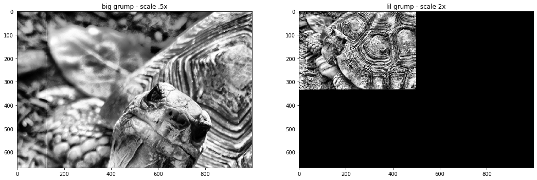
As you can tell, this will scale the whole image from the origin point of 0, 0. We can designate the origin point through these matrices as well!
\begin{bmatrix} X & OriginY & 0 \\ OriginX & Y & 0 \\ 0 & 0 & 1 \end{bmatrix}
But let’s not rest on our matrix laurels, grump demands more transformation explorations! Let’s examine what scaling is doing to our numpy array, in a crude way – to make the image bigger, we’re selecting or cropping a segment of the image and stretching that smaller crop out, ‘zooming in’ on that segment until it fills the original image’s dimensions.
And to make the image smaller, we’re adding some proportional number of empty rows and columns to our image array, and resizing it to the original image’s dimensions. We add whitespace and downscale the image, ‘zooming out’.
if we follow this thinking through, using some functions from scikit-image util and transfrom modules, we’ll have a centered and scaled image!
#'zooming in'
def scale_grump(image, scalex, scaley):
    '''scale grump using our atypical description!'''
    mod_img = image
    if scalex < 1:
        scale_boundx = int(((1-scalex) * image.shape[1]) // 2)
        mod_img = skimage.util.crop(mod_img, ((1, 1), (scale_boundx, scale_boundx)))
        mod_img = skimage.transform.resize(mod_img, (image.shape[0], image.shape[1]))

    if scaley < 1:
        scale_boundy = int(((1-scaley) * image.shape[0]) // 2)
        mod_img = skimage.util.crop(mod_img, ((scale_boundy, scale_boundy), (1, 1)))
        mod_img = skimage.transform.resize(mod_img, (image.shape[0], image.shape[1]))

    #'zooming out' by padding edges with a proportional scale value, array will be filled with 0's (blk)
    if scalex > 1:
        #use padding to rescale img
        paddingx = int(((scalex - 1) * image.shape[1]) // 2)
        mod_img = skimage.util.pad(mod_img, pad_width = ((0, 0), (paddingx, paddingx)), mode = 'constant', constant_values = 0)
        mod_img = skimage.transform.resize(mod_img, (image.shape[0], image.shape[1]))

    if scaley > 1:
        paddingy = int(((scaley - 1) * image.shape[0]) // 2)
        mod_img = skimage.util.pad(mod_img, pad_width = ((paddingy, paddingy), (0, 0)), mode = 'constant', constant_values = 0)
        mod_img = skimage.transform.resize(mod_img, (image.shape[0], image.shape[1]))

    return np.float32(mod_img)
lil_grump = scale_grump(adapthist, 2, 2) #making a half-sized grump
big_grump = scale_grump(adapthist, .9, .5) #scaling x by a small amount, y by double!

#small grump, rescaled back to original size using the same technique
returned_grump = scale_grump(lil_grump, .5, .5)

plt.figure(figsize = (18, 8))
plt.subplot(1,3,1)
plt.imshow(lil_grump, cmap = 'gray')
plt.title('lil grump')
plt.subplot(1,3,2)
plt.imshow(big_grump, cmap = 'gray')
plt.title('big grump')
plt.subplot(1,3,3)
plt.imshow(returned_grump, cmap = 'gray')
plt.title('returned grump')
plt.show()
plt.imshow(returned_grump - adapthist, cmap = 'gray')
plt.title('returned grump minus original image')
plt.show()
print('you see some differences in values on the final img due to interpolation during the downsize / upsizing of the image')


Shear
We’ll do one final transform – the dreaded shear! *shudder*
Make that grumpy tortoise quake in his boots… shell… whatever! Shear can be used as another matrix transform, but as usual, we’ll get there another way. The following is for a horizontal (x-axis) shear, where theta represents the newly created interior angle of the side and the moved axis’s furthest point (don’t stress it if it doesn’t make sense yet!) :
\begin{bmatrix} 1 & tan\theta & 0 \\ 0 & 1 & 0 \\ 0 & 0 & 1 \end{bmatrix}But constructing our own matrices is so blasé. We’re moving on to more scikit-image
functions that will do it for us!:
skimage.transform.AffineTransform()
Shear values given to this function will be in counter-clockwise radians; remember that 1 radian is nearly 60 degrees, so most of these values will be very small.
Also, I’m getting tired of all these gray image plots – we can spice things up, tortoise style! All our images are still black and white, but we can use different color maps in pyplot.
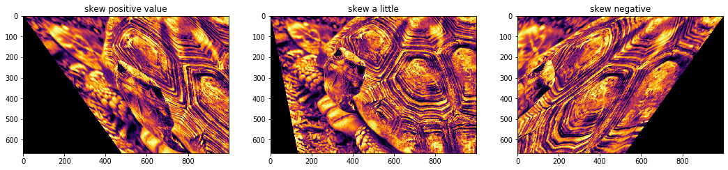
matrix = skimage.transform.AffineTransform(scale = (1.0, 1.0), rotation = 0, shear = .8)
matrix_inv = skimage.transform.AffineTransform(scale = (1.0, 1.0), rotation = 0, shear = -.8)
matrix_small = skimage.transform.AffineTransform(scale = (1.0, 1.0), rotation = 0, shear = .2)

plt.figure(figsize=(18, 8))
plt.subplot(1,3,1)
plt.imshow(skimage.transform.warp(adapthist, matrix), cmap = 'inferno')
plt.title('skew positive value')
plt.subplot(1,3,2)
plt.imshow(skimage.transform.warp(adapthist, matrix_small), cmap = 'inferno')
plt.title('skew a little')
plt.subplot(1,3,3)
plt.imshow(skimage.transform.warp(adapthist, matrix_inv), cmap = 'inferno')
plt.title('skew negative')
plt.show()
And we’re still using the transform module’s warp function, which means different modes!
plt.figure(figsize=(18, 8))
plt.subplot(1,3,1)
plt.imshow(skimage.transform.warp(adapthist, matrix, mode = 'symmetric'), cmap = 'inferno')
plt.title('symmetric mode')
plt.subplot(1,3,2)
plt.imshow(skimage.transform.warp(adapthist, matrix, mode = 'edge'), cmap = 'inferno')
plt.title('edge mode')
plt.subplot(1,3,3)
plt.imshow(skimage.transform.warp(adapthist, matrix, mode = 'wrap'), cmap = 'inferno')
plt.title('wrap mode')
plt.show()

Skew can be especially useful when compensating for or dealing with differences in image perception due to perspective. It’s a fast, simple process that can do a lot to remove (or add) image distortion.
That covers all of the transform operations that we’ll need to move on to image dataset augmentation, but we have one more process that is definitely worth a couple more code cells! These are not transforms but are:
Noise & Blur
Adding in visual noise and blurring an image can make a big difference on a neural network’s ability to generalize, so we’ll take a minute to go over gaussian blur and adding noise.
noise_sm = skimage.util.random_noise(adapthist, mode = 'gaussian', mean = 0, var = .05)
noise_md = skimage.util.random_noise(adapthist, mode = 'speckle', mean = 0, var = 3)
noise_lg = skimage.util.random_noise(adapthist, mode = 'poisson')

print('Different Noise types:')
plt.figure(figsize=(18, 8))
plt.subplot(1,3,1)
plt.imshow(noise_sm, cmap = 'gray')
plt.title('Gaussian Grump')
plt.subplot(1,3,2)
plt.imshow(noise_md, cmap = 'gray')
plt.title('Speckled Grump')
plt.subplot(1,3,3)
plt.imshow(noise_lg, cmap = 'gray')
plt.title('Poisson Grump')
plt.show()

OK, we can speckle this tortoise and swing it around, so let’s get on to the last piece and blur it up!
focus1_grump = skimage.filters.gaussian(adapthist, sigma = 2, mode = 'nearest', preserve_range = True)
focus2_grump = skimage.filters.gaussian(adapthist, sigma = 7, mode = 'nearest', preserve_range = True)
focus3_grump = skimage.filters.gaussian(adapthist, sigma = 15, mode = 'nearest', preserve_range = True)

print('Gaussian Blur')
plt.figure(figsize=(18, 8))
plt.subplot(1,3,1)
plt.imshow(focus1_grump, cmap = 'gray')
plt.title('blurry')
plt.subplot(1,3,2)
plt.imshow(focus2_grump, cmap = 'gray')
plt.title('blurrier')
plt.subplot(1,3,3)
plt.imshow(focus3_grump, cmap = 'gray')
plt.title('blurriest')
plt.show()
